Circuit QED (Part 2)
Part 2: The coplanar waveguide resonator
In Part 1 I discussed the superconducting quantum LC oscillator, which will form the foundation for much of the rest of this series. What I did not discuss, though, is how such a circuit is actually constructed. Although it is easy to understand theoretically, it turns out that it’s pretty difficult to make an ideal LC circuit on a superconducting chip. In practice, most circuit QED experiments use a structure called the coplanar waveguide resonator, or CPW. The CPWs are the squiggly bits on our LEGO model:
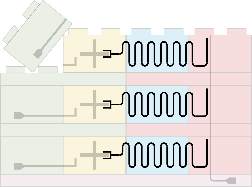
In this post we will take an in-depth look at what these are and how they work. At the end of Part 1 I said that one cannot build a qubit from an LC circuit alone, and the same is true for the CPW. However, the CPW is an integral part of many circuit QED devices. As we will see in a later post, it facilitates qubit readout, among other things. The CPW will also provide us with our first direct link between the math of quantum mechanics and a real, physical device – and one that’s surprisingly simple at that. Lastly, by the end of this post, we will be ready to address a question that you might have had this whole time: Why is it called circuit QED?
From thin films to quantum fields
A coplanar waveguide is basically just what you get if you take a length of coaxial cable and make it flat (or coplanar). Instead of a center conductor separated from a coaxial outer conductor by a layer of insulating material, it is constructed from a thin metal film deposited on an insulating substrate; a center conductor is then separated from the rest of the film. The substrate is typically silicon or sapphire, while the superconducting film is typically aluminum, niobium, or tantalum. The factors that go into the choice of materials is far beyond the scope of this post. For now I’ll just say that this choice involves a tradeoff between multiple factors such as the desired noise properties of the device, ease of fabrication, and compatibility with other materials in the device.
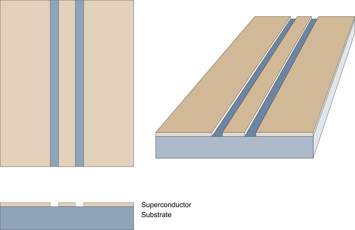
Note that this figure is not to scale. The width of the center conductor relative to its separation from the rest of the film affects the CPW’s properties, and here I just chose something that looks reasonable. Also, the relative thicknesses of the superconducting film and the substrate are vastly different from what is shown here: the film is generally a few tens to hundreds of nanometers thick, while the substrate is generally around half a millimeter thick. Finally, for the rest of this post I will stick with the top-down view. The 3D figure is helpful in explaining the basic geometry of the device, but my Inkscape skills are not up to the task of making the remaining figures in 3D.
Building intuition
My goal here is of course to describe the CPW in a fairly rigorous way. First, though, let’s develop some intiution. Imagine that we have a CPW oriented along the \(x\) axis, which starts at \(x = 0\) and extends to \(x \rightarrow \infty\). We connect a voltage source at \(x = 0\) and apply a signal \(V(t)\):
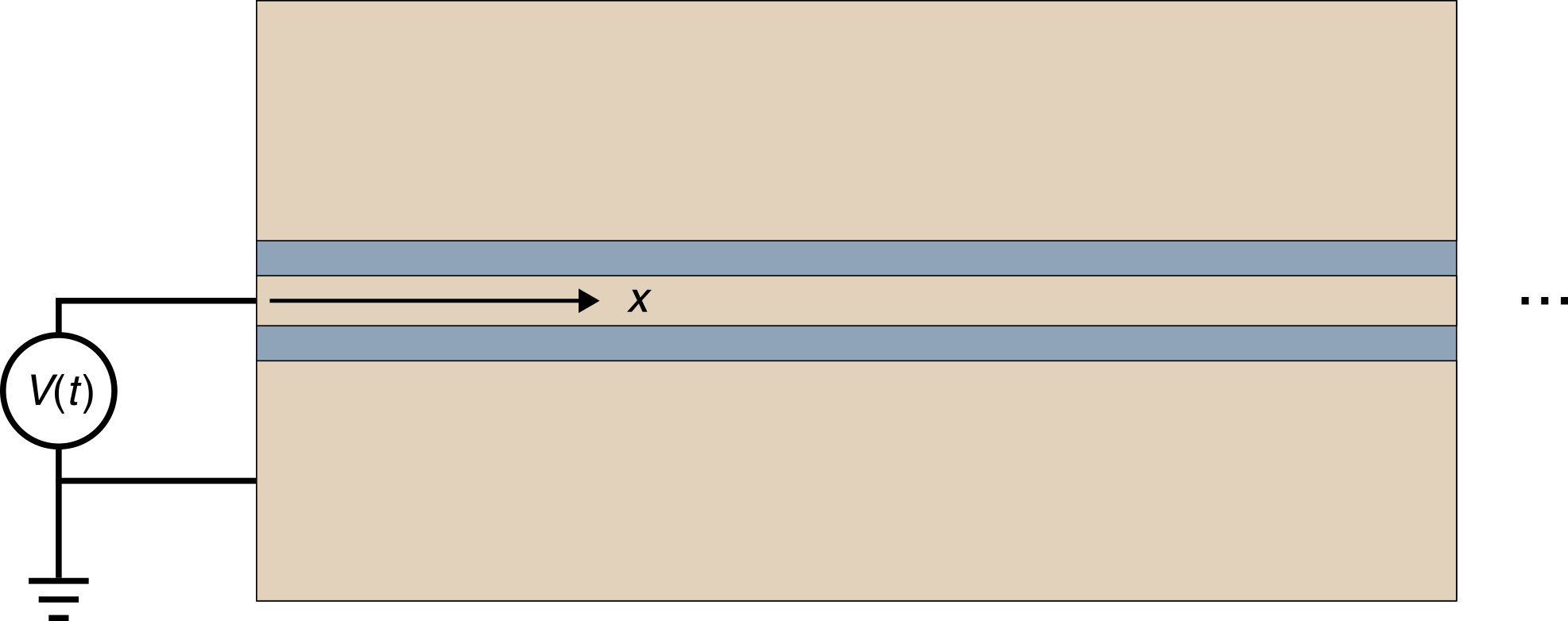
Let’s say this voltage signal is \(V(t) = V_0 \cos(\omega t)\). What is the voltage measured at a position \(x\) along the CPW, \(V(x, t)\)? We know that \(V(0, t) = V_0 \cos(\omega t)\). We could reasonably guess that the system behaves like a coaxial cable, in the sense that the signal propagates down it at some speed \(v_0\). In this case the voltage has the form of a propagating wave:
where \(k = \omega / v_0\).
The main point I want to make here is that the coplanar waveguide, as its name suggests, supports waves of oscillating voltage and current. When the length of the waveguide extends to infinity, the wavelength – or equivalently, frequency – can take any value (up to a point, anyway: the waveguide stops behaving like a one-dimensional structure when the wavelength becomes comparable to its transverse dimensions). On the other hand, suppose we introduce some boundary conditions by, for example, introducing “breaks” in the CPW:
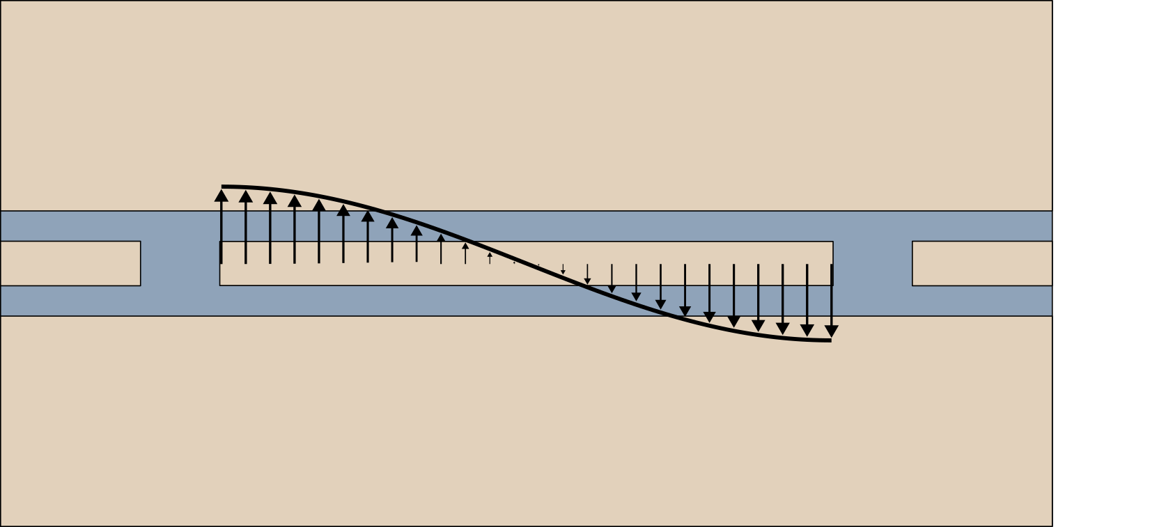
Like sound waves in a length of pipe, the vibrations of a guitar string, or the oscillating currents in an antenna, the voltage along the CPW forms a number of standing waves – or “normal modes” – whose wavelengths are commensurate with the boundary conditions. In this case, the breaks at the two ends mean that we have current nodes and voltage antinodes at the boundaries. The standing wave mode shown here is the one with the longest wavelength, which is twice the length of the section of CPW. We therefore refer to this as a \(\lambda/2\) resonator. Had we instead grounded both ends, we would still have a \(\lambda/2\) resonator, but with the nodes and antinodes reversed. Grounding one end and leaving the other open yields a \(\lambda/4\) resonator.
Here is a microscope image (the very first in this series!) of a CPW resonator on one of our chips, coupled to a feedline (bottom) and a transmon qubit (top):
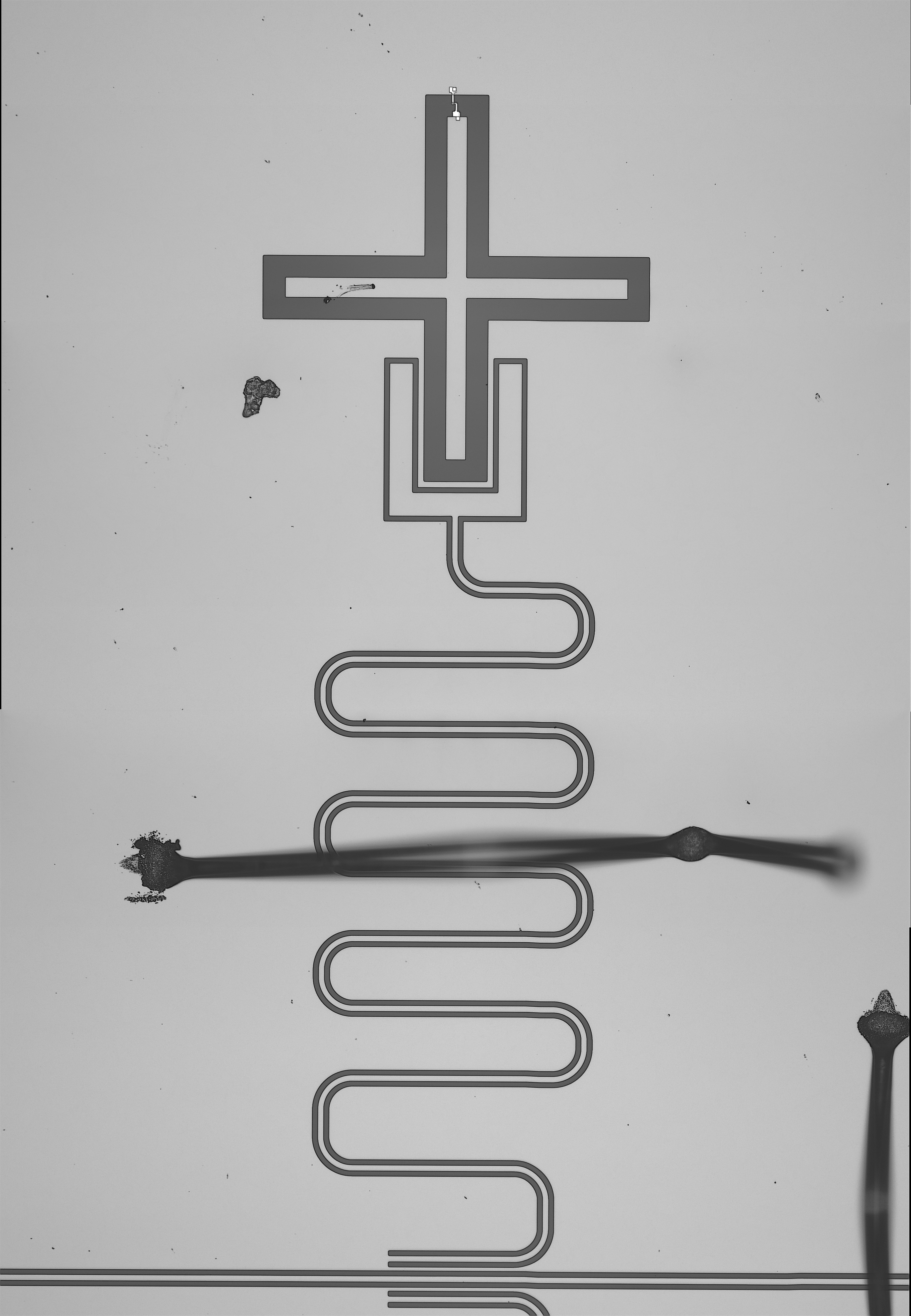
The big ugly thing across the image is a wire bond, which serves to bridge the ground planes on either side of the resonator. The CPW is designed with this meandering shape in order to make it take up less space on the chip. The “U”-shaped “claw” at the top serves to capacitively couple it to the transmon qubit (the “+”-shaped thing). If you look closely at the ends of the resonator, you’ll notice that the end at the bottom is connected to the surrounding ground plane, while the end at the top is floating. This is therefore a \(\lambda/4\) resonator, which is a common choice for this application because we want its footprint on the chip to be as small as possible.
It is at this point that astute readers might begin to suspect that these standing wave modes have something to do with the quantum harmonic oscillator. In a normal mode, voltages and currents in the CPW resonator will oscillate back and forth in time at some characteristic frequency. So perhaps if we cool the circuit down and treat it quantum mechanically, it will act as the real-life counterpart to the quantum LC oscillator of the previous post…
The telegrapher model
Our general approach to quantizing this system will be the following:
- Ask the electrical engineers for an equivalent circuit model for the system.
- Use this circuit model to write down a Lagrangian, from which we identify canonically conjugate variables.
- Perform a Legendre transform to obtain the Hamiltonian.
- Promote the canonically conjugate variables to operators and diagonalize the Hamiltonian.
The circuit model describing a coplanar waveguide is called the telegrapher model. It consists of a chain of infinitesimal inductors and capacitors:
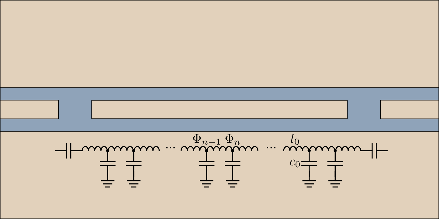
A single cell of this chain has a length \(\delta x\). The \(l_0\) and \(c_0\) are the inductance and capacitance per unit length of the chain, so that the inductance of each cell is \(L_0 = \delta x l_0\) and its capacitance is \(C_0 = \delta x c_0\). To see the origin of this model, consider a short segment of the CPW. It clearly has some capacitance to ground, being a piece of metal separated from the ground plane. The value of this capacitance per unit length is a function of the geometry of the CPW and the dielectric constant of the insulating substrate. Meanwhile, if we consider a current flowing through this chunk of CPW, it is clear that it should generate some circulating magnetic field. This magnetic field will in turn resist changes in the current flowing through the chunk, and this is the origin of the inductance. See e.g. Ref. [1] for analytic solutions for the capacitance and inductance per unit length in terms of the waveguide geometry and substrate dielectric constant.
We proceed by finding the inductive and capacitive energies associated with each unit cell. You will notice in the previous figure that the fluxes \(\Phi_n\) are associated with the nodes of the circuit (the connections between the inductors and capacitors, not “nodes” in the wave sense used above). This may seem a bit strange, as the actual fluxes in the circuit are through the inductors. However, it will turn out to be a very convenient choice. The flux through the inductor between nodes \(n - 1\) and \(n\) is \(\Phi_n - \Phi_{n-1}\). Thus the inductive energy associated with unit cell \(n\) is
If node \(n\) has a charge \(Q_n\), its capacitive energy is
The relationship between \(\Phi_n\) and \(Q_n\) is essentially what we would expect: because voltage is the time derivative of flux through an inductor, and because the charge on a capacitor is its capacitance times the voltage across it, we have
There are actually several subtleties here, mainly residing in the difference between “node variables” and “branch variables.” Rather than become bogged down in this formalism, I will simply refer you to Michel Devoret [2].
Provided that you believe me or, failing that, believe Professor Devoret, we can proceed with writing down the Lagrangian for the system. Because the inductive part is the “potential energy” and the capacitive part is the “kinetic energy,” we have
where \(N\) is the total number of unit cells. Next we take the continuum limit. Dividing out a factor of \(\delta x\), the Lagrangian becomes
We define a charge density field \(Q(x)\), a flux field \(\Phi(x)\), and take the limit \(\delta x \rightarrow 0\) while keeping \(N \delta x\) fixed to obtain
where we have assumed that the waveguide extends from \(x = 0\) to \(x = D\), and we have used the limit definition of the derivative for the \(\partial_x \Phi(x)\) term. The integrand here is a quantity known in field theory as the Lagrangian density, \(\mathcal{L}(x)\). Taking \(\Phi(x)\) to be the “position” field, we find the canonically conjugate momentum field in the usual way:
and noting that in the continuum limit our above result for \(\partial_t \Phi_n\) implies that \(Q(x) = c_0 \partial_t \Phi(x)\), we find
that is, the charge density field is the conjugate momentum to the flux field.
We transform from a Lagrangian density to a Hamiltonian density by performing a Legendre transform. For a classical (non-field) system the Legendre transform for a system with position variable \(\phi\) and conjugate momentum variable \(p\) is
and it works the same in field theory for the Lagrangian density and Hamiltonian density. Substituting our conjugate pair, we have
which yields
The total Hamiltonian is found by integrating the Hamiltonian density:
Canonical quantization of the eigenmodes
At this point, most authors would proceed by finding the classical equation of motion describing the field in the CPW, solving for its eigenmodes, and then promoting the conjugate variables defining each eigenmode to canonically conjugate observables. The Hamiltonian can then be diagonalized in the usual manner, and we would be justified in saying that we are finished.
If it hasn’t become clear yet, I sometimes like to introduce things in an unorthodox way. I won’t claim that it’s better, but maybe it’s at least interesting. In any case, for the sake of completeness I will present both this path and an alternative one, starting with the usual treatment.
The classical equation of motion can be found in either the Lagrangian or Hamiltonian picture. I will choose the former. The Euler-Lagrange equation for a 1D scalar field is
This looks a little different from the Euler-Lagrange equation you might be used to from the classical mechanics of particles, but it has the same origin: it gives an extremum of the time integral of the Lagrangian, i.e., the action. I give a derivation of this equation in the Appendix.
In the present case of a massless scalar field, the third term on the left vanishes. We write the Lagrangian density in terms of \(\Phi\),
and take the various derivatives and rearrange slightly to find
This is the wave equation! The wave’s speed is evidently \(v_0 = 1 / \sqrt{l_0 c_0}\). In practice this speed turns out to be somewhere around a third of the speed of light in vacuum, where the specific proportionality constant depends on the dielectric constant of the insulating substrate and the fraction of the electric field that lives in the substrate. Writing the wave equation in terms of this speed:
The solutions to the wave equation are, of course, waves. It is helpful to separate the time dependence from the spatial dependence, writing a generic solution for wavenumber \(k\) as
where \(A_k\) is a normalization constant, \(\phi_k\) is is a phase offset to be determined by the boundary conditions, and the frequency and wavenumber are related by \(\omega_k = v_0 k\). Here we have neglected an irrelevant phase shift on the time-dependent term.
Now we introduce boundary conditions. Suppose the resonator extends from \(x = 0\) to \(x = D\) and has open boundary conditions at both ends (i.e. neither end of the resonator is connected to ground). This forces the current through the waveguide to be zero at the boundaries. It is not too hard to see from the circuit model that the current is related to the flux field by
which implies that we have a discrete set of solutions, which we index by \(m = 0, 1, 2, \ldots\):
and \(\phi_m = 0\). You can work out the solutions for other boundary conditions for yourself.
We call these solutions “normal modes.” The overall field can be decomposed into normal modes:
where \(\Phi_m(t)\) oscillates at the normal mode frequency \(\omega_m = v_0 k_m\) and
We determine the normalization constant by requiring that
from which one obtains \(A_m = \sqrt{2/D}\). This choice of normalization has the consequence that we can write
which is why it’s such a convenient choice.
If we re-express the Lagrangian of the system in terms of the normal modes, we have
which, after taking advantage of the fact that the normal modes are orthogonal and normalized, simplifies to
The conjugate momentum to the generalized coordinate \(\Phi_m\) is therefore \(Q_m = c_0 \partial_t \Phi_m\), and a Legendre transform yields a Hamiltonian consisting of a sum of independent harmonic oscillators:
I will note that if you compare this to, e.g., the Blais et al. review [3], you will find a slight discrepancy. In that review, the normalization condition is defined to be
This causes the Hamiltonian to have factors of \(C_r = c_0 D\) in place of the \(c_0\) in my version. Both versions are equivalent, differing by a choice of dimensions for the generalized positions and momenta. The physics is unchanged by this choice, and I feel that the form I presented here will make the connection to the second approach (given below) more clear.
We now proceed with quantization. When we “canonically quantize” a system, all that means is that we replace classical position variables and their conjugate momenta with observable operators satisfying the canonical commutation relation:
or setting \(\hbar = 1\),
In Part 1 I simply asserted that flux and charge play the roles of position and momentum and imposed the canonical commutation relation on them without justifying it. If you were left feeling a bit uncertain about that procedure, I hope this clears things up. We now have our Hamiltonian operator,
which consists of infinitely many decoupled harmonic oscillators and can therefore be diagonalized in the usual way. We write annihilation and creation operators for each mode,
and
and the Hamiltonian can be rewritten as
The factor of \(\frac {\omega_m} {2}\) looks rather problematic. It suggests that, even when every harmonic oscillator is in its ground state, the system has infinite energy (since we’re summing the ground state energy \(\frac {\omega_m} {2}\) over all \(m\)). This is the ultraviolet divergence of quantum field theory, and I don’t have much to say about it that hasn’t been said before. The discussion in David Tong’s lecture notes is quite approachable, and in any case, it is clear that in our system the summation over \(m\) should not be taken to infinity in the first place. For high enough frequencies (that is, short enough wavelengths) the waveguide stops behaving like a waveguide. Moreover, as discussed briefly in Part 1, we shouldn’t allow for modes whose energies are comparable to or larger than the superconducting gap energy.
So, that’s that. We started with a circuit model, wrote down a Lagrangian, transformed to a Hamiltonian, and applied canonical quantization to the normal modes. The result is a system of many decoupled quantum harmonic oscillators. In practice, we would typically make use of just a single mode (usually the lowest-frequency/longest-wavelength one), pretending that the other ones don’t exist. This is generally a very good approximation: for a \(\lambda/2\) resonator the frequency of the first harmonic is twice that of the fundamental, which is more than far enough away to safely be ignored. This is where most discussions of CPW resonators for circuit QED would move on to their various applications and complications, and we could certainly do that here.
However, I would like to leave the discussion of applications for another post, and instead look at the waveguide from a different perspective – that of quantum field theory.
A massless 1D scalar quantum field
In the approach given above, we applied canonical quantization to the normal modes of the resonator. What if we instead applied it to the field itself?
Recall that we had the flux field, \(\Phi(x)\), and its conjugate momentum, \(Q(x)\). We can just promote these to observable operators, \(\hat{\Phi}(x)\) and \(\hat{Q}(x)\), with the canonical commutation relation
It is important to understand that we now have an operator-valued field, where each position \(x\) has its own Hilbert space, completely separate from any other position \(x'\). If we were to write a wavefunction for some state of the system, it would not have the form \(\psi(x)\). Rather, it would assign an amplitude to every possible configuration of the entire field. The position \(x\) becomes a label specifying which “part of the Hilbert space” we’re looking at, rather than an observable operator as in standard quantum mechanics.
We can define other operators in terms of the field operators. For example, the normal mode operators are given by
and
You can check for yourself that these definitions give rise to the expected commutation relation \([\hat{\Phi}_m, \hat{Q}_{m'}] = i \delta_{m,m'}\).
The normal modes are special because they block-diagonalize the Hamiltonian, turning it into a collection of independent harmonic oscillators. In other situations, however, other types of collective modes may be more useful. For example, one might want to think about collections of left- or rightward propagating modes which carry information into or away from a device [4,5], or between devices [6]. One can even have multiple propagating modes with very specific temporal profiles which can overlap while remaining orthogonal to one another [7].
Beyond its usefulness for things like quantum state transfer, I just think this is cool. We have a sort of “synthetic” quantum field, one coming from the quantized motion of the flux and charge distributed throughout a device made according to our specifications. In particular, it is a massless 1D scalar field – massless due to the lack of a \(\Phi(x)\) term without derivatives in the Lagrangian, and scalar because (classically) the field takes a single scalar value at each position (…and I trust that the 1D part is obvious enough). This is sort of the simplest possible quantum field, the thing usually given as a first example in a QFT course. The only fundamental scalar field that has been observed so far is the Higgs field, but this is a massive scalar field.
With that being said, the field we have here is sort of analogous to what you get if you restrict the electromagnetic field to one dimension. Quantum electrodynamics is the theoretical framework describing the quantized electromagnetic field and its interactions with matter. Superconducting qubits are “artificial atoms” because, as we will see, they consist of a number of bound energy eigenstates which interact with the quantized electromagnetic field in a CPW or in an actual 3D cavity. Circuit QED reproduces classic QED effects like the Lamb shift, and the calculations we do in this field often very closely resemble those performed when considering the interaction of the electromagnetic field and matter.
The power of circuit QED, and much of its draw for people like me, is that we get all of this physics in a system that we design. Our “atoms” are not limited to those of the periodic table. Rather, there is a vast landscape of possible superconducting qubits, and nearly any Hamiltonian you can think up can be realized through some combination of circuit elements and control pulses. Likewise, we can achieve extremely strong light-matter interactions through the design of the device itself. In this way, more than just being a viable platform for quantum computation, superconducting circuits present us with a rich and exciting means of experimentally probing aspects of quantum physics that might otherwise remain beyond our reach – and the humble coplanar waveguide will be found in just about every one of these experiments.
Appendix: The Euler-Lagrange equation for a 1D scalar field
The reason that the Euler-Lagrange equation for the field looks a little weird basically comes down to the fact that \(x\) is not a generalized coordinate in the way that a particle’s position is in the standard Lagrangian mechanics of particles. Rather, it is a sort of label that indexes distinct generalized coordinates \(\Phi(x)\). We begin by writing the action, i.e., the time integral of the Lagrangian:
where \(\mathcal{L}(x)\) is really a function of \(\Phi(x)\), \(\partial_x \Phi(x)\), and \(\partial_t \Phi(x)\). We find the equations of motion for the system by requiring that the action is stationary. That is, for a small variation \(\delta \mathcal{L}\) which keeps the end points fixed, the corresponding variation in the action is zero: \(\delta S = 0\). The variation can be written as
so that
The latter two terms can be integrated by parts to yield
Notice that the second integral involves the total derivatives, and so the requirement that the variation vanishes at the end points causes the entire integral to vanish. We are left with
The requirement that the variation of the action vanishes for all possible start and end points means that, for the whole integral to always vanish, the integrand itself must vanish. Thus,
which is equivalent to the Euler-Lagrange equation given above.
Finally, I won’t go through it here, but it would be a fun exercise to start with the discretized circuit model for the resonator,
and, treating each \(\Phi_n\) as a distinct generalized coordinate, apply the usual Euler-Lagrange equation to determine the equations of motion. Following this, take the limit as \(\delta x \rightarrow 0\), keeping the total length of the resonator fixed as we did before, and see that you once again recover the wave equation.
- S. Gevorgian, L. J. P. Linner, and E. L. Kollberg, CAD models for shielded multilayered CPW, IEEE Transactions on Microwave Theory and Techniques 43, 772 (1995).
- M. H. Devoret, Quantum Fluctuations in Electrical Circuits, in Fluctuations Quantiques/Quantum Fluctuations, edited by S. Reynaud, E. Giacobino, and J. Zinn-Justin (1997), p. 351.
- A. Blais, A. L. Grimsmo, S. M. Girvin, and A. Wallraff, Circuit quantum electrodynamics, Rev. Mod. Phys. 93, 025005 (2021).
- M. P. da Silva, D. Bozyigit, A. Wallraff, and A. Blais, Schemes for the observation of photon correlation functions in circuit QED with linear detectors, Phys. Rev. A 82, 043804 (2010).
- C. Eichler, D. Bozyigit, C. Lang, L. Steffen, J. Fink, and A. Wallraff, Experimental State Tomography of Itinerant Single Microwave Photons, Phys. Rev. Lett. 106, 220503 (2011).
- A. Almanakly et al., Deterministic remote entanglement using a chiral quantum interconnect, Nature Physics 21, 825 (2025).
- A. Hernández-Antón, J. D. Schär, A. Grigorev, G. F. Peñas, R. Puebla, J. J. García-Ripoll, J.-C. Besse, A. Wallraff, and A. Kulikov, Emission and Absorption of Microwave Photons in Orthogonal Temporal Modes across a 30-Meter Two-Node Network, (2026).