The Hitchhiker’s Guide to Circuit QED (Part 1)

Part 1: The quantum LC oscillator

In November of 2025, the Blok lab celebrated the successful PhD defense of one of the first students to join the group, Mihirangi Medahinne. It was a bittersweet moment. On the one hand, Mihi was the first student from the lab to graduate – a milestone for any research group. On the other hand, it’s always a bit sad seeing a colleague leave, even if they’re destined for bigger and better things. Hers was the first project I worked on when I joined the group, and I gained a great deal of knowledge about nanofabrication (and eventually coauthorship on a publication [1]) from the experience.

In her PhD defense talk, Mihi compared fabricating superconducting circuit devices to building with LEGOs. I think it’s a great analogy. Most circuit quantum electrodynamics (circuit QED) experiments are built from a handful of components, arranged and designed to interact with each other in new and creative ways.

In Part 2 I will introduce one of these LEGO bricks: the coplanar waveguide resonator. Part 3 will introduce the transmon qubit. Nearly everything I will discuss in this series is based on these components.

Before we talk about resonators and qubits, though, it’s helpful to look at an even simpler device: the LC oscillator. This circuit will be the focus of this post, and as we will see, it lays the groundwork for everything that is to come.

Quantizing a circuit

Consider a capacitor with capacitance $C$ and an inductor with inductance $L$ in parallel:

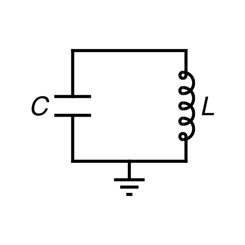
We’d like to analyze what happens when we quantize this circuit. This may seem like a strange idea. Electrical circuits are macroscopic devices, and their operation involves the motion of an enormous number of electrons. We’re used to thinking of quantum systems as being small, and as being comprised of a relatively small number of particles.

This is where the “superconducting” in “superconducting circuits” comes in. A superconductor is a material in which all of the free electrons occupy a single quantum ground state. In short, this is possible because, in certain materials at low temperatures, pairs of electrons become bound to one another in what is known as a Cooper pair. We learn in introductory quantum mechanics that electrons are fermions, and that fermions obey the Pauli exclusion principle: no two fermions can occupy the same quantum state. Cooper pairs, however, effectively behave as bosons. This property allows every Cooper pair in the material to occupy the same quantum ground state. The electrons’ wavefunctions become delocalized throughout the material, and so long as nothing causes them to become excited – to break a Cooper pair – they flow through the material without dissipation.

I realize that this explanation of superconductivity leaves a lot to be desired. As I said in the introduction to this series, I do not plan to talk much about superconductivity itself. If you’re interested in learning more, the theory describing the formation of Cooper pairs is called the Bardeen-Cooper-Schrieffer (BCS) theory.

Moving on: the key point is that, if our electrical circuit is constructed from a superconductor, then the whole thing exists in one big coherent quantum state. We are free to analyze the quantum behavior of the circuit in terms of its macroscopic degrees of freedom, namely, the charge difference $Q$ across the capacitor and the flux $\Phi$ threading the inductor. Recall from your introductory electricity and magnetism course that the energy stored in a capacitor is given by $Q^2 / 2C$, while that stored in an inductor is $\Phi^2 / 2L$. We can somewhat arbitrarily decide that the capacitive part of the energy plays the role of “kinetic energy” (with the charge being the “momentum”), and the inductive part plays the role of “potential energy” (with the flux being the “position”). This choice doesn’t matter much right now, but its utility will become clear when we discuss qubits.

These “position” and “momentum” variables form a conjugate pair, and we quantize the system by promoting them to non-commuting observables:

$$ [\hat{\Phi}, \hat{Q}] = i \hbar. $$

Here we make a choice regarding units. In circuit QED we typically work in units where $\hbar = 1$, because it allows us to use angular frequency and energy interchangeably, and because we don’t want a bunch of $\hbar$s everywhere. I will stick with this convention throughout this series because I like it and I’m used to it.

We can now write the Hamiltonian describing our LC circuit:

$$ \hat{H}_{\rm LC} = \frac {1} {2C} \hat{Q}^2 + \frac {1} {2L} \hat{\Phi}^2. $$

Clearly this Hamiltonian represents a quantum harmonic oscillator: the kinetic energy is quadratic in the momentum variable, and the potential energy is quadratic in the position variable. We follow the usual procedure of diagonalizing the Hamiltonian in terms of an annihilation operator $\hat{a}$ and a creation operator $\hat{a}^\dagger$:

$$ \hat{\Phi} = \left ( \frac {L} {4 C} \right )^{1/4} \left ( \hat{a}^\dagger + \hat{a} \right ) \equiv \Phi_{\rm zpf} \left ( \hat{a}^\dagger + \hat{a} \right ) $$

and

$$ \hat{Q} = i \left ( \frac {C} {4 L} \right )^{1/4} \left ( \hat{a}^\dagger - \hat{a} \right ) \equiv i Q_{\rm zpf} \left ( \hat{a}^\dagger - \hat{a} \right ). $$

Notice that all of the quantities which are not dimensionless are contained in the zero-point fluctuations $\Phi_{\rm zpf}$ and $Q_{\rm zpf}$. The creation and annihilation operators obey the commutation relation

$$ [\hat{a}, \hat{a}^\dagger] = 1, $$

which is easily shown by writing them in terms of $\hat{\Phi}$ and $\hat{Q}$ and making use of the canonical commutation relation given above. Substituting into the Hamiltonian we find

$$ \hat{H}_{\rm LC} = \sqrt{\frac {1} {LC}} \left ( \hat{a}^\dagger \hat{a} + \frac {1} {2} \right ), $$

and we see that – as we should expect from the classical case – the oscillator’s frequency is

$$ \omega_{\rm LC} = \sqrt{\frac {1} {LC}}, $$

so we write

$$ \hat{H}_{\rm LC} = \omega_{\rm LC} \left ( \hat{a}^\dagger \hat{a} + \frac {1} {2} \right ). $$

I will generally adopt the convention of dropping the constant factor of $1/2$ from the Hamiltonian, because it has no effect on the dynamics of the system. Finally, then,

$$ \hat{H}_{\rm LC} = \omega_{\rm LC} \hat{a}^\dagger \hat{a}. $$

It is useful to define the number operator, which gives the number of excitations in the oscillator: $\hat{N} = \hat{a}^\dagger \hat{a}$.

Rather than continue to work out the properties of the Hamiltonian and the creation and annihilation operators (also called “ladder operators”), I will simply state a few of them. The details can be found in any introductory quantum mechanics text.

We denote the eigenstates of the system (also commonly called “Fock states”) by $|n\rangle$, where $n = 0, 1, 2, \ldots$. The effect of the annihilation operator is to annihilate an excitation: $\hat{a} |n\rangle = \sqrt{n} |n - 1\rangle$ (who would’ve thought?). The creation operator similarly creates an excitation: $\hat{a}^\dagger |n\rangle = \sqrt{n + 1} |n + 1\rangle$. The creation and annihilation operators are clearly not Hermitian, and thus not observables.

The eigenenergies $\omega_n$ of the system are given by evaluating $\hat{H}_{\rm LC} |n\rangle$, which yields

$$ \omega_n = n \omega_{\rm LC}. $$

That is, our quantum LC circuit, like any other quantum harmonic oscillator, has infinitely many energy eigenstates, with energies that are integer multiples of the resonant frequency of the circuit. We will explore the consequences of this below.

But first, let’s take a step back. We started with a macroscopic electrical circuit, and by building that circuit from a superconducting material, we are able (or so I claim) to think of it as a coherent quantum mechanical system. In particular, the parallel LC circuit realizes a quantum harmonic oscillator, where charge is the analog of momentum and flux is the analog of position. Under what conditions is this picture actually valid?

As with any system, the quantum effects become significant at low energies. The first question, then, is how low the energy can be – how close can we get to the ground state? Intuitively, we should expect that the system is in its ground state when its temperature is low enough that it cannot be thermally excited. Concretely, the ratio of the population in the first excited state of the oscillator to that in the ground state is given by the Boltzmann distribution:

$$ \frac {P(|1\rangle)} {P(|0\rangle)} = \exp \left [-\frac {\hbar \omega_{\rm LC}} {k_B T} \right ], $$

so the system is in the ground state when $\hbar \omega_{\rm LC} \gg k_B T$. A typical dilution refrigerator reaches temperatures around 10 mK. Substituting this value and the constants we find that the condition is $\omega_{\rm LC} / 2\pi \gg 200$ MHz, and so we have a lower bound on the required resonant frequency. For frequencies lower than this, there is significant thermal population in the oscillator’s excited states. There are ways of dealing with this, and sometimes in circuit QED we do design oscillators and qubits with lower frequencies, knowing that we’ll have to deal with thermal excitation. Still, this provides a rough order-of-magnitude estimate for how low the resonant frequency could reasonably be.

At the other extreme, we must be careful that the energy required to excite the oscillator does not affect the superconductor itself. The energy required to excite an electron from the collective ground state is called the superconducting gap, and its value varies quite a lot depending on the material used and the thickness of the film. As an estimate let’s take the superconducting gap for thin-film aluminum to be on the order of $\Delta = 200$ μeV. The energy required to break a Cooper pair is twice this value, because both electrons must be excited. Setting $\hbar \omega_{\rm LC} \ll 2 \Delta$ we find $\omega_{\rm LC} / 2\pi \ll 100$ GHz.

To summarize, we must simultaneously satisfy the constraint imposed by the temperature of the fridge, $\omega_{\rm LC} / 2\pi \gg 200$ MHz, and that imposed by the superconducting gap, $\omega_{\rm LC} / 2\pi \ll 100$ GHz. We typically choose frequencies on the order of 1 - 10 GHz for these reasons, as well as the fact that experimental instruments (oscillators, waveform generators, oscilloscopes, and so on) that operate in this frequency range are easy to come by. As far as equipment is concerned, going to lower frequencies is not much of a problem. But once you go past 10 GHz, generating control pulses can become seriously problematic (read: expensive).

Having hopefully convinced you that it’s valid to think of the superconducting LC circuit as a quantum harmonic oscillator, let’s continue to explore its properties.

Following the usual steps for the quantum harmonic oscillator, one finds that the eigenstate wavefunctions in the flux basis are

$$ \psi_n(\phi) = c_n e^{-\frac {1} {4} \left ( \frac {\phi} {\Phi_{\rm zpf}} \right )^2 } H_n \left ( \frac {1} {\sqrt{2}} \frac {\phi} {\Phi_{\rm zpf}} \right ) $$

where $H_n(x)$ is a Hermite polynomial. I’ll plot these wavefunctions on top of the quadratic potential well. The vertical offset of each wavefunction indicates its eigenenergy.

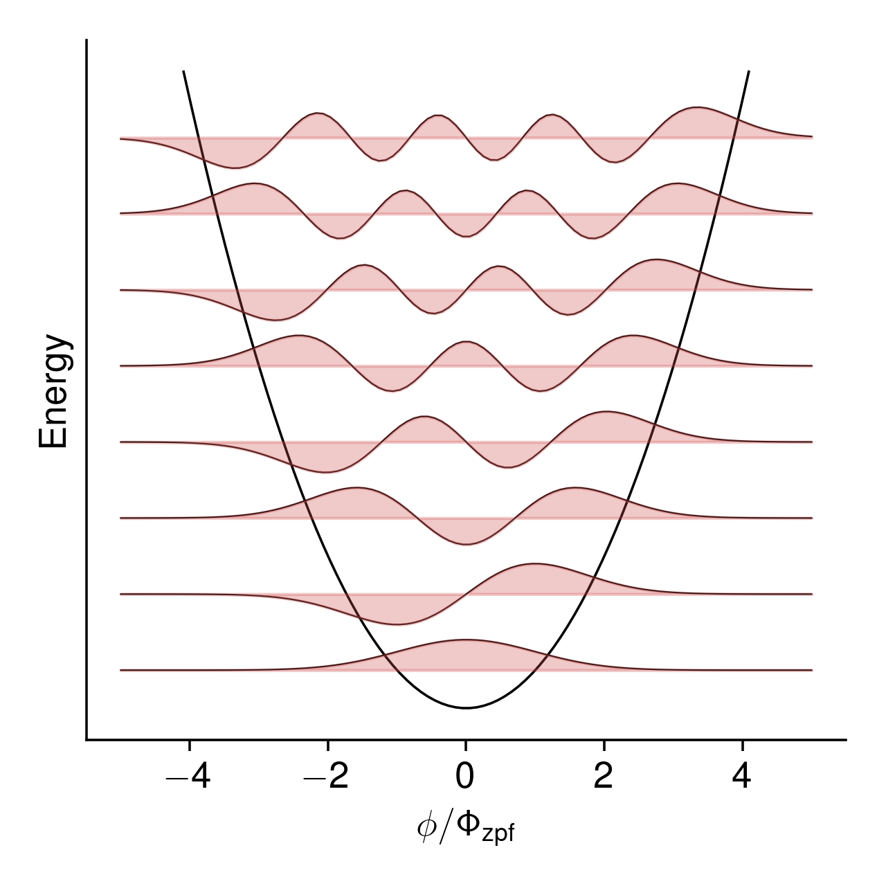
There’s a lot we could talk about here, but I’ll focus on two things: zero-point fluctuations and the classical limit of the system. First, look at the ground state wavefunction. Classically, we would expect that the lowest-energy state of the circuit is the one with zero charge and zero flux. Quantum mechanically, however, the ground state wavefunction has some “spread” – some probability of finding the circuit in a state with nonzero flux. The same holds true for charge. This is the meaning of the zero-point flucuations, also known as vacuum fluctuations: even in its lowest-energy state, the charge and flux of the oscillator are fluctuating in the sense that, when we measure them, they can take nonzero values. Looking again at the $\Phi_{\rm zpf}$ and $Q_{\rm zpf}$ given above:

$$ \Phi_{\rm zpf} = \left ( \frac {L} {4 C} \right )^{1/4} $$

and

$$ Q_{\rm zpf} = \left ( \frac {C} {4 L} \right )^{1/4}, $$

we see that they are inversely related: as the ratio of inductance to capacitance changes, so too does the ratio of the zero-point fluctuations. We will return to this idea in Part 3.

Next, let’s consider the classical limit. It’s tempting to imagine that we get a “classical” state of the system by going to a very high-energy eigenstate, because we typically imagine classical mechanics as being the high-energy limit of quantum mechanics. But a classical state should be one where the circuit has a single, definite charge, and a single, definite flux. The energy eigenstates, on the other hand, are all smeared out.

This begs the question: what type of state does become “classical” in the high-energy limit? As most readers who have studied quantum mechanics will know, the answer to this question is the collection of states known as coherent states. Coherent states will come up several times over the course of this series, so it’s worthwhile to discuss them now.

Coherent states

Coherent states are often introduced as being the eigenstates of the annihilation operator:

$$ \hat{a} |\alpha\rangle = \alpha |\alpha\rangle, $$

where $\alpha$ is any complex number. While mathematically straightforward, I feel that this definition contains little physical insight. What does it mean for something to be an eigenstate of the annihilation operator? We can come up with reasonable and interesting answers to this question, but it doesn’t feel like a good starting point to me.

Instead, let’s imagine the type of transformation that we should do to the system in order to take it from its ground state to a “classical” state. On a physical level, we do this by adding some charge to the capacitor, adding some flux to the inductor, or both. Our task is to describe this procedure mathematically. What we’re looking for is a unitary transformation $\hat{D}(\Delta \phi, \Delta q)$ that takes the system from an initial state with flux $\phi$ and charge $q$ to a final state with flux $\phi + \Delta \phi$ and charge $q + \Delta q$. Applying this transformation to the ground state of the oscillator and taking the limit of large $\Delta \phi$ and/or large $\Delta q$ will give us our classical state.

To construct such an operator, consider displacing an arbitrary wavefunction $\psi(\phi)$ by a small amount, $\delta \phi$. To lowest order we can write the displaced state as

$$ \psi_{\delta \phi}(\phi) = \psi(\phi - \delta \phi) \approx \left (1 - \delta \phi \frac {d} {d\phi} \right ) \psi(\phi). $$

Recalling from intro QM that the “momentum” is given in the “position” basis as $q = -i \frac {d} {d\phi}$:

$$ \psi_{\delta \phi}(\phi) \approx \left (1 - i \delta \phi q \right ) \psi(\phi). $$

In the limit $\delta \phi \rightarrow 0$, this equation becomes exact. Moving away from the wavefunction language, we can now write the displacement operator for an infinitesimal displacement:

$$ \hat{D}(\delta \phi, 0) \approx 1 - i \delta \phi \hat{Q}. $$

Now imagine that we want to displace the state by some larger amount, $\Delta \phi$. We can do this by breaking $\Delta \phi$ into $N$ infinitesimal pieces $\Delta \phi / N$, and displacing by this amount $N$ times. Thus

$$ \hat{D}(\Delta \phi, 0) = \lim_{N \rightarrow \infty} \left (1 - i \frac {\Delta \phi} {N} \hat{Q} \right )^N, $$

which is just another way of writing the exponential:

$$ \hat{D}(\Delta \phi, 0) = e^{-i \Delta \phi \hat{Q}}. $$

A more formal way of stating this is that the charge operator is the generator of displacements in flux. The flux operator is likewise the generator of displacements in charge. Ultimately, the operator that generates an arbitrary displacement in both variables is

$$ \hat{D}(\Delta \phi, \Delta q) = e^{-i \left ( \Delta \phi \hat{Q} - \Delta q \hat{\Phi} \right )}. $$

The more common form of the displacement operator is written in terms of the ladder operators:

$$ \begin{split} \hat{D}(\Delta \phi, \Delta q) &= e^{-i \left ( \Delta \phi i Q_{\rm zpf} \left ( \hat{a}^\dagger - \hat{a} \right ) - \Delta q \Phi_{\rm zpf} \left ( \hat{a}^\dagger + \hat{a} \right ) \right )} \\ &= e^{\left (\Delta \phi Q_{\rm zpf} + i \Delta q \Phi_{\rm zpf} \right ) \hat{a}^\dagger - \left (\Delta \phi Q_{\rm zpf} - i \delta q \Phi_{\rm zpf} \right ) \hat{a}}, \end{split} $$

or defining the complex coordinate $\alpha \equiv \Delta \phi Q_{\rm zpf} + i \Delta q \Phi_{\rm zpf}$,

$$ \hat{D}(\alpha) = e^{\alpha \hat{a}^\dagger - \alpha^* \hat{a}}. $$

Our classical states are those obtained by applying a displacement to the ground state:

$$ |\alpha\rangle = \hat{D}(\alpha) |0\rangle. $$

Showing that these are the same coherent states that we obtain from the usual definition, $\hat{a} |\alpha\rangle = \alpha |\alpha\rangle$, is a fun little exercise which I will leave to you (hint: Baker-Campbell-Hausdorff formula). Or you can just take my word for it.

Expanding a coherent state $|\alpha\rangle$ in the Fock basis yields

$$ |\alpha\rangle = e^{-\frac {|\alpha|^2} {2}} \sum_n \frac {\alpha^n} {\sqrt{n!}} |n\rangle, $$

meaning that the distribution of Fock states in a coherent state is Poissonian.

One can furthermore show that they have the following properties:

The average number of excitations in a coherent state is $\langle \alpha | \hat{N} | \alpha \rangle = |\alpha|^2$.
The variance of the number of excitations in a coherent state is also $|\alpha|^2$, which means that its uncertainty is $\Delta \hat{N} = |\alpha|$. This means that the relative uncertainty is $\Delta \hat{N} / \langle \hat{N} \rangle = 1 / |\alpha|$, which approaches zero as the size of the coherent state becomes large.
The coherent states form an overcomplete basis (i.e., they are not orthogonal to one another).
Applying a displacement to a coherent state always yields another coherent state, up to a global phase:

$$ \hat{D}(\beta) |\alpha\rangle = e^{(\beta \alpha^* - \beta^* \alpha) / 2} |\alpha + \beta\rangle. $$

Phew. I know that was a lot of boring math, and I hope you’ll accept my sincere apologies. The good news is that now things are getting fun.

First, let’s explore this idea that the coherent states form an overcomplete basis. That coordinate, $\alpha$, can take any value on the complex plane. Let’s see what happens when we use this property to help us visualize other quantum states. For any arbitrary state $|\psi\rangle$, let’s define a function

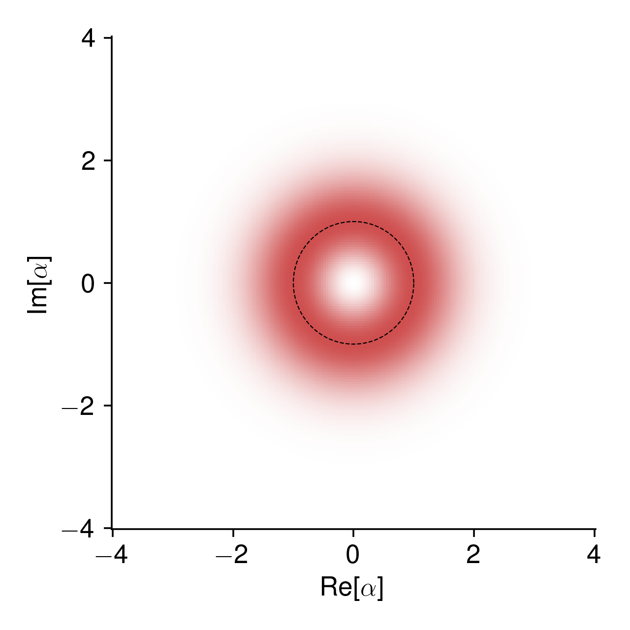
$$ \mathcal{Q}_{|\psi\rangle}(\alpha) = |\langle \alpha | \psi \rangle |^2. $$

We’ll take this function and plot it using color on a 2D plane, where the horizontal axis is the real part of $\alpha$ (corresponding to the flux coordinate of the oscillator) and the vertical axis is the imaginary part (corresponding to charge). Let’s start with a simple example: the ground state. Clearly we have

$$ \mathcal{Q}_{|0\rangle}(\alpha) = e^{-|\alpha|^2}, $$

i.e., a Gaussian distribution (up to normalization). Plotting this:

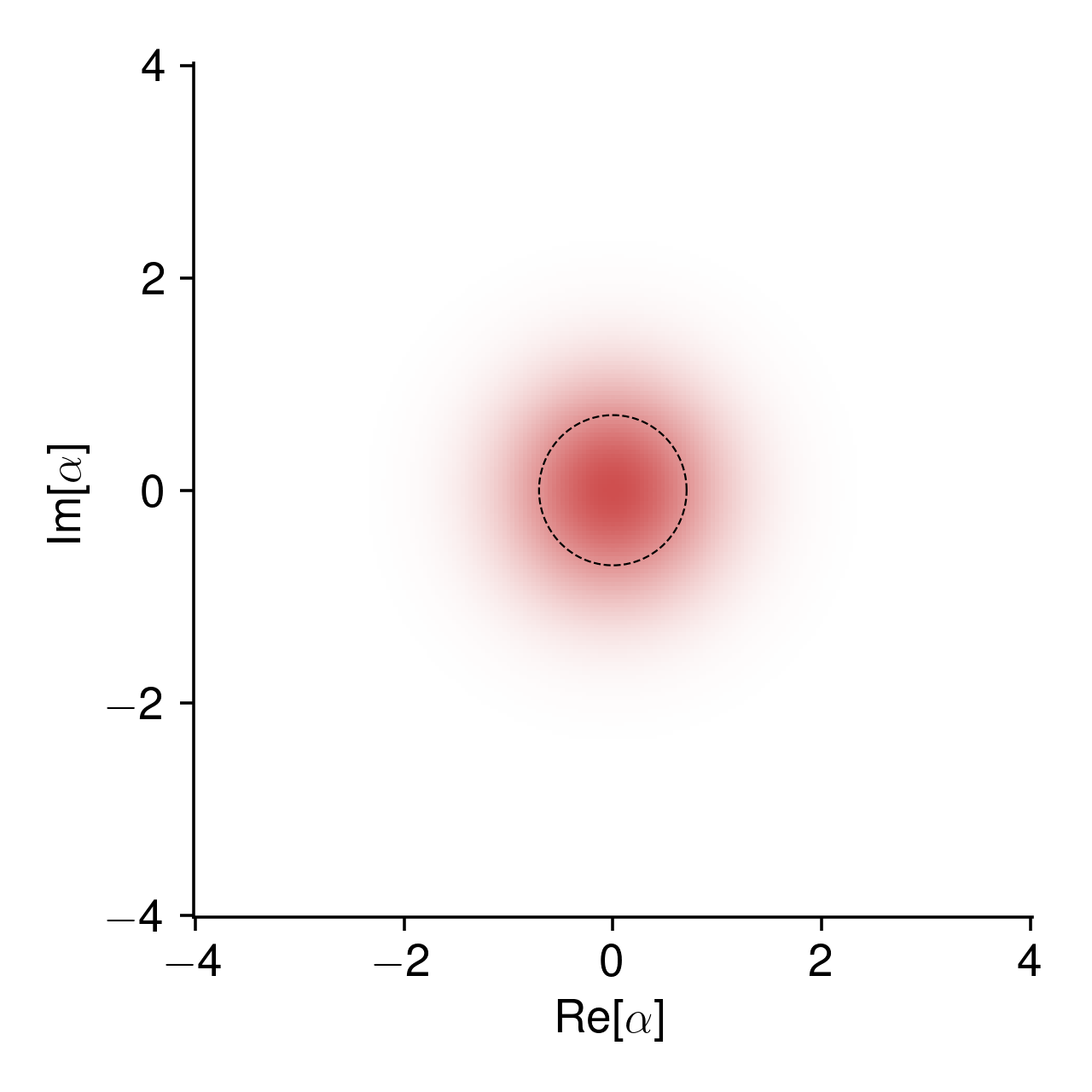
The dashed circle is $|\alpha| = 1/\sqrt{2}$, the characteristic size of the zero-point fluctuations when translated into phase space coordinates.

Next let’s look at what we get for some other coherent states $|\beta\rangle$. For $\beta = 4$:

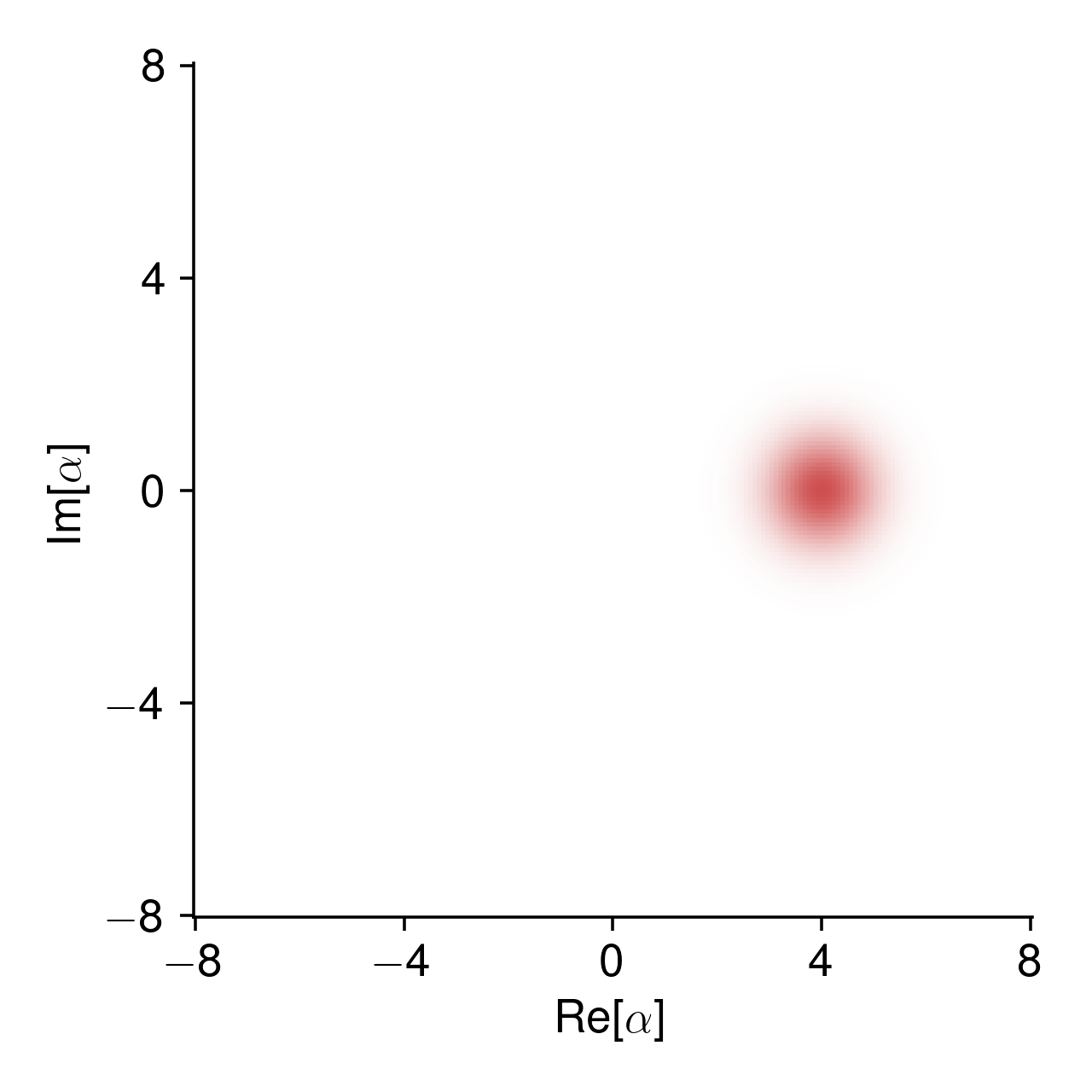
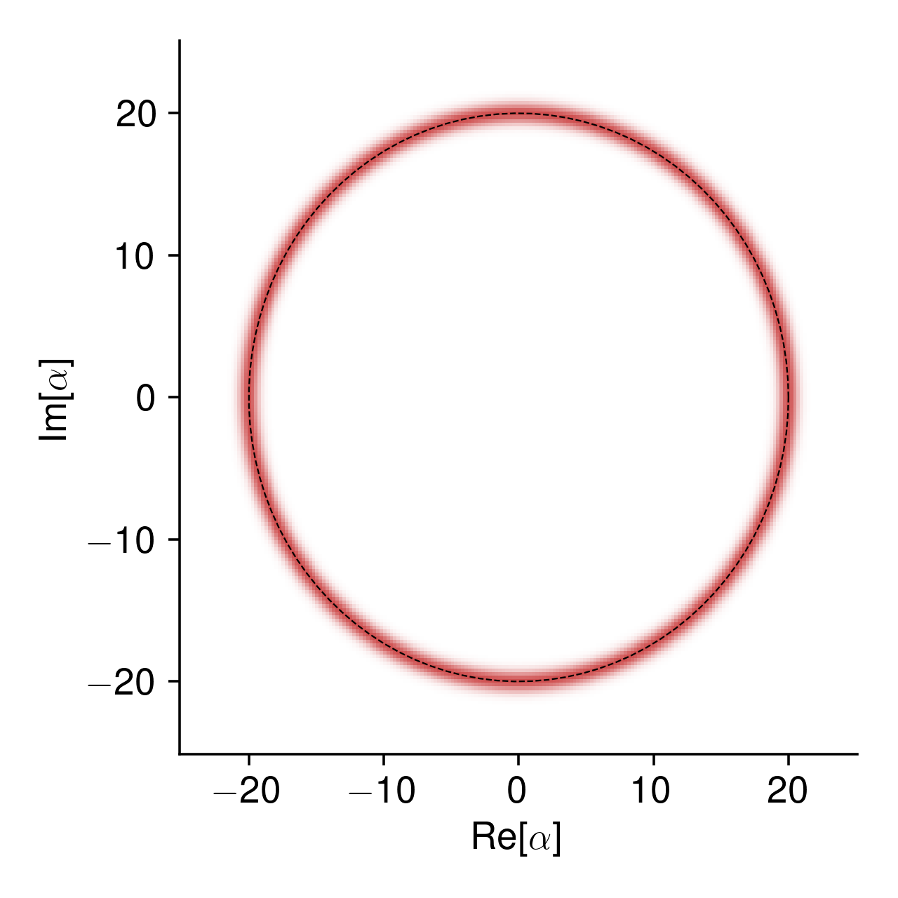
Notice that I’ve rescaled the axes. The size of the “blob” hasn’t changed, but its apparent size relative to its displacement from the origin has decreased. For $\beta = 20$:

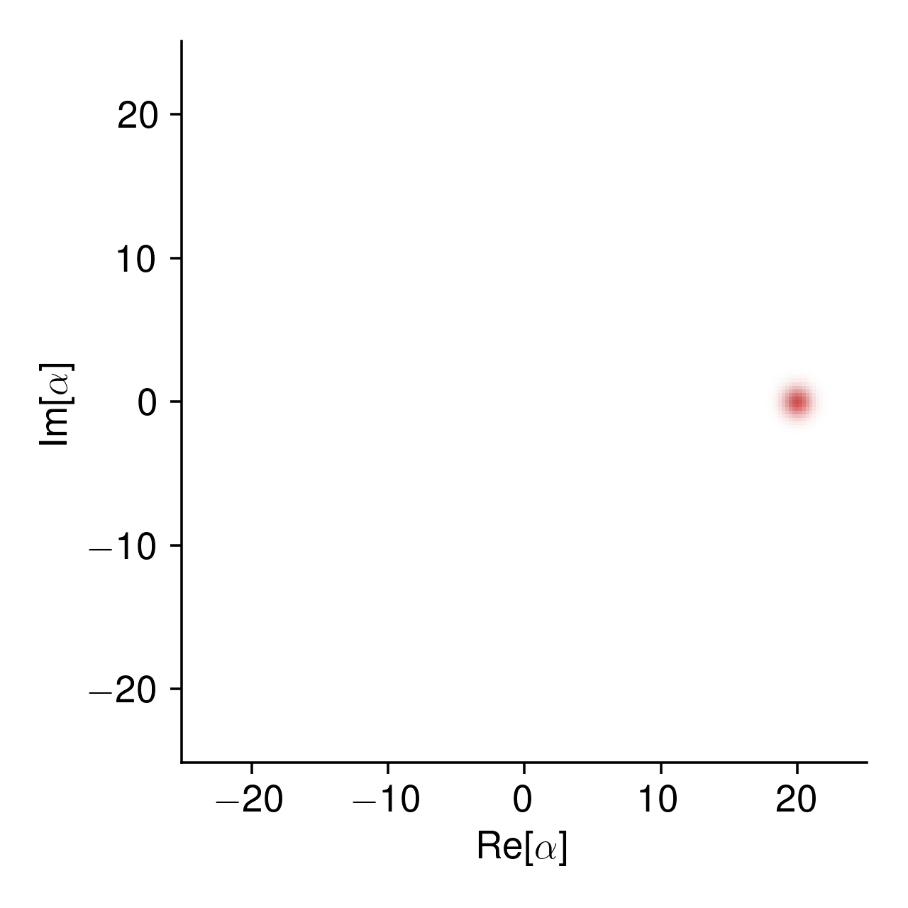
Before long, the state stops looking smeared out at all. As we displace our coherent state further and further from the origin, it begins to look more and more like a single point – like a classical state, with a definite flux and definite charge in the circuit.

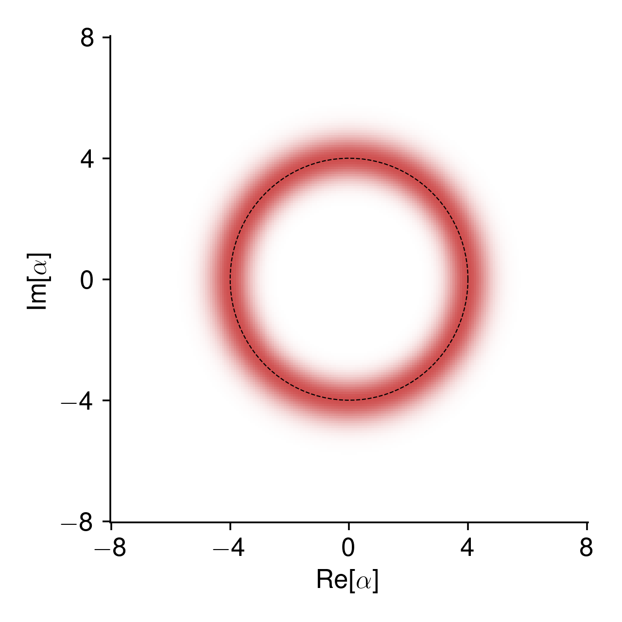
The Fock states, on the other hand, look very different. For the first excited state of the oscillator, Fock state $|1\rangle$, we get:

In these plots the dashed line indicates $|\alpha| = \sqrt{n}$. For $|16\rangle$:

And for $|400\rangle$:

We can understand this behavior by going back to our LC oscillator Hamiltonian:

$$ \hat{H}_{\rm LC} = \frac {1} {2C} \hat{Q}^2 + \frac {1} {2L} \hat{\Phi}^2. $$

We can take a classical limit by simply replacing our charge and flux operators with regular old classical numbers, thereby obtaining an energy surface:

$$ E(Q, \Phi) = \frac {1} {2C} Q^2 + \frac {1} {2L} \Phi^2. $$

We translate to our dimensionless phase space coordinate $\alpha$:

$$ {\rm Re}[\alpha] = \Phi Q_{\rm zpf}, $$

$$ {\rm Im}[\alpha] = Q \Phi_{\rm zpf}, $$

and we ultimately find

$$ E(\alpha) = \omega_{\rm LC} |\alpha|^2. $$

How do we interpret this? For a given classical energy $E$, there is a continuous ring of points in phase space, $\alpha$, where the system could be. In other words, knowing the energy alone is not enough to determine the charge and flux – we only know that the system must lie on a ring in phase space. The radius of this ring is given by the (square root of) the ratio of the energy to the resonant frequency of the oscillator. In the quantum mechanical case, then, it makes perfect sense that energy eigenstates – where only the energy is known – would be smeared out along this ring.

We can visualize other types of states in this way too. For example, here’s what the state $\frac {1} {\sqrt{2}} (|0\rangle + |3\rangle)$ looks like:

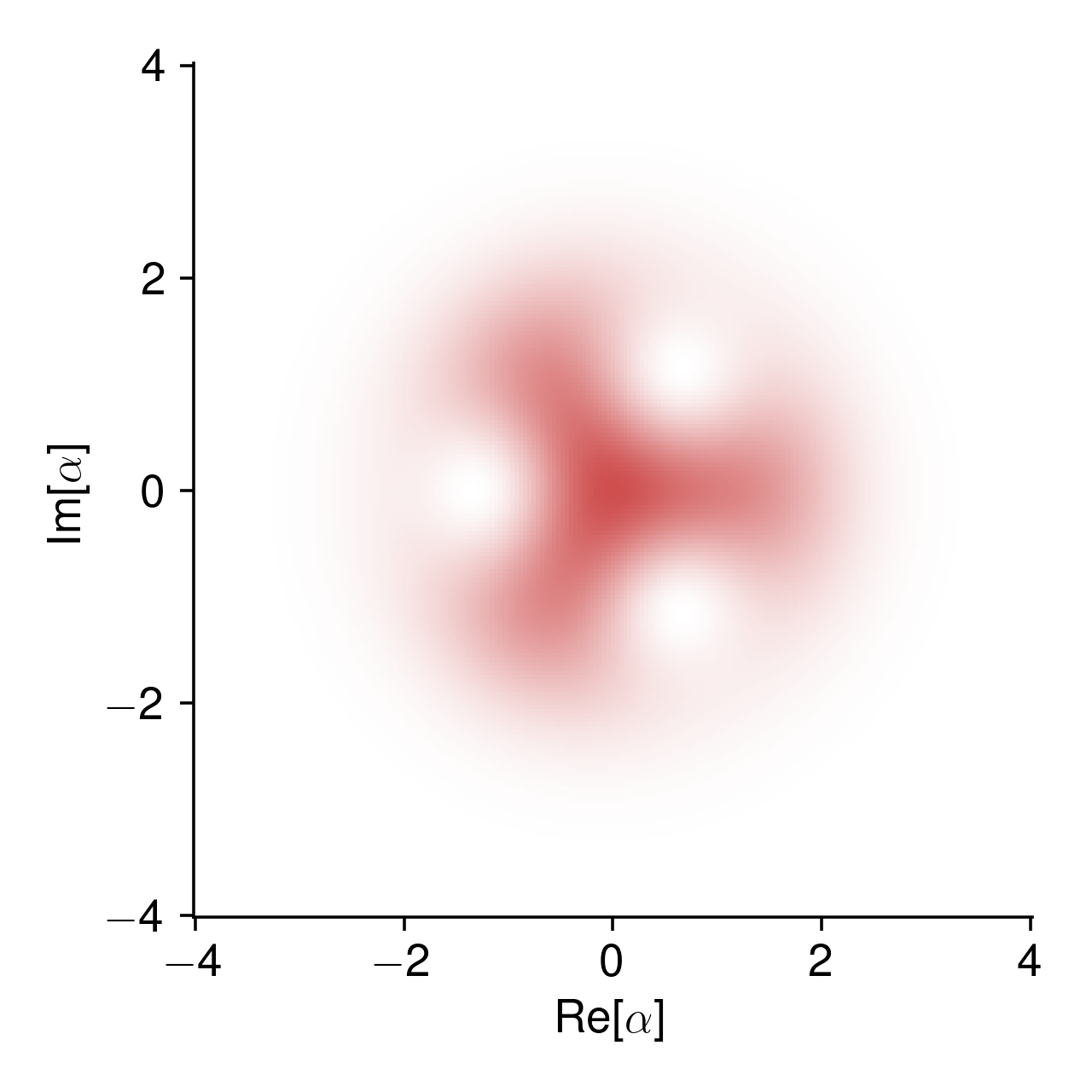
See if you can convince yourself of why it should have this three-fold rotational symmetry.

This function, $\mathcal{Q}_{|\psi\rangle}(\alpha)$, is known as the Husimi Q function (usually it has a normalization factor of $1/\pi$). More than just a fun visualization, it is a ubiquitous tool in experimental quantum optics and circuit QED, because it is a physically measurable quantity. To see one way that we could measure it, note that $\langle \alpha | = \langle 0 | \hat{D}^\dagger(\alpha)$. Therefore, we apply a displacement of $\hat{D}^\dagger(\alpha) = \hat{D}(-\alpha)$ to the state in the oscillator and measure the resulting population in the ground state by doing many shots of the experiment and recording the fraction of them that yield $|0\rangle$ (for now I’m intentionally leaving it vague as to exactly how this measurement is done). The information contained in the Q function completely determines the state, and so it serves as a means of tomographically reconstructing the state of the oscillator. Lastly, I will note that the Q function is an example of a broader class of quasiprobability distributions in phase space, another example of which is the Wigner distribution.

Time dynamics

Conspicuously missing from our discussion so far is the fact that, in general, the state of the oscillator will evolve in time. Considering the classical version of the problem, suppose we start at $t = 0$ with some charge $Q_0$ on the capacitor and zero flux in the inductor. What happens next?

Solving the equation of motion of the system, we will find that the charge oscillates back and forth:

$$ Q(t) = Q_0 \cos(\omega_{\rm LC}t). $$

The energy is tranferred into flux:

$$ \Phi(t) = -Q_0 \sqrt{\frac {L} {C}} \sin(\omega_{\rm LC} t). $$

Stated another way, the system evolves along the constant-energy rings in phase space.

How does this play out in the quantum mechanical case? Time evolution in quantum mechanics is generated by the Hamiltonian through the Schrodinger equation:

$$ \frac {d |\psi(t)\rangle} {dt} = -i \hat{H}(t) |\psi(t)\rangle. $$

When the Hamiltonian is time-independent, the solution is conveniently given through its exponentiation:

$$ |\psi(t)\rangle = e^{-i \hat{H} t} |\psi(0)\rangle. $$

In our case the Hamiltonian is $\omega_{\rm LC} \hat{a}^\dagger \hat{a}$. This is easy to exponentiate because it’s diagonal. Written in the Fock basis,

$$ e^{-i \omega_{\rm LC} \hat{a}^\dagger \hat{a} t} = e^{-i \omega_{\rm LC} \sum_n n |n\rangle \langle n| t} = \sum_n e^{-i n \omega_{\rm LC} t} |n\rangle \langle n|. $$

If we want to compare the time evolution of the system to the classical case, then we should begin in a coherent state. For an arbitrary initial coherent state $|\alpha\rangle$, we substitute our Fock-basis expression from above:

$$ \begin{split} |\psi(t)\rangle &= \left ( \sum_n e^{-i n \omega_{\rm LC} t} |n\rangle \langle n| \right ) |\alpha\rangle \\ &= \left ( \sum_n e^{-i n \omega_{\rm LC} t} |n\rangle \langle n| \right ) \left ( e^{-\frac {|\alpha|^2} {2}} \sum_n \frac {\alpha^n} {\sqrt{n!}} |n\rangle \right ) \\ &= e^{-\frac {|\alpha|^2} {2}} \sum_n \frac {\left ( e^{-i \omega_{\rm LC} t} \alpha \right ) ^n} {\sqrt{n!}} |n\rangle \\ &= |e^{-i \omega_{\rm LC} t} \alpha \rangle. \end{split} $$

That is, our state remains a coherent state, which rotates about the origin in phase space at a frequency $\omega_{\rm LC}$.

Next we take the expectation value of the charge operator:

$$ \begin{split} \langle \hat{Q}(t) \rangle &= \langle e^{-i \omega_{\rm LC} t} \alpha | \hat{Q} | e^{-i \omega_{\rm LC} t} \alpha \rangle \\ &= \langle e^{-i \omega_{\rm LC} t} \alpha | i Q_{\rm zpf} \left ( \hat{a}^\dagger - \hat{a} \right ) | e^{-i \omega_{\rm LC} t} \alpha \rangle \\ &= i Q_{\rm zpf} \left ( \langle e^{-i \omega_{\rm LC} t} \alpha | \hat{a}^\dagger | e^{-i \omega_{\rm LC} t} \rangle - \langle e^{-i \omega_{\rm LC} t} | \hat{a} | e^{-i \omega_{\rm LC} t} \alpha \rangle \right ) \\ &= i Q_{\rm zpf} \left ( e^{i \omega_{\rm LC} t} \alpha^{*} - e^{-i \omega_{\rm LC} t} \alpha \right ) \\ &= 2 Q_{\rm zpf} {\rm Im} \left [ e^{-i \omega_{\rm LC} t} \alpha \right ] \end{split} $$

Setting $\langle \hat{Q}(0) \rangle = Q_0$, so that we can compare with the classical case, we see that

$$ \alpha = \frac {i Q_0} {2 Q_{\rm zpf}} $$

and therefore

$$ \langle \hat{Q}(t) \rangle = Q_0 \cos(\omega_{\rm LC}t), $$

just like the classical case. For flux, meanwhile,

$$ \begin{split} \langle \hat{\Phi}(t) \rangle &= \langle e^{-i \omega_{\rm LC} t} \alpha | \hat{\Phi} | e^{-i \omega_{\rm LC} t} \alpha \rangle \\ &= \langle e^{-i \omega_{\rm LC} t} \alpha | \Phi_{\rm zpf} \left ( \hat{a}^\dagger + \hat{a} \right ) | e^{-i \omega_{\rm LC} t} \alpha \rangle \\ &= \Phi_{\rm zpf} \left ( \langle e^{-i \omega_{\rm LC} t} \alpha | \hat{a}^\dagger | e^{-i \omega_{\rm LC} t} \rangle + \langle e^{-i \omega_{\rm LC} t} | \hat{a} | e^{-i \omega_{\rm LC} t} \alpha \rangle \right ) \\ &= \Phi_{\rm zpf} \left ( e^{i \omega_{\rm LC} t} \alpha^{*} + e^{-i \omega_{\rm LC} t} \alpha \right ) \\ &= 2 \Phi_{\rm zpf} {\rm Re} \left [ e^{-i \omega_{\rm LC} t} \alpha \right ] \\ &= -Q_0 \frac {\Phi_{\rm zpf}} {Q_{\rm zpf}} \sin(\omega_{\rm LC}t) \\ &= -Q_0 \sqrt{\frac {L} {C}} \sin(\omega_{\rm LC}t). \end{split} $$

For coherent states, then, the expectation values of the charge and flux operators give us a correspondence between the quantum and classical pictures. Importantly, in the quantum case there will be some variance to these expectation values, coming from the zero-point fluctuations. But as the amplitude of the coherent state (i.e., the initial charge or flux in the circuit) is increased, the relative sizes of these fluctuations decrease.

Final thoughts

So far, I haven’t really talked about how a superconducting quantum LC oscillator is actually physically realized on a chip. This will be the topic of Part 2, where I will discuss coplanar waveguide resonators.

For now, I hope I have convinced you that, at least in principle, building an LC circuit from superconducting materials gives us a quantum harmonic oscillator. And by cooling it to a temperature well below the energy scale set by its resonant frequency, it reaches its quantum ground state. To wrap this post up, I want to focus on the following question: can we use an LC circuit to build a qubit?

I suppose that I should first define what a “qubit” is. A qubit is a two-level quantum mechanical system which forms the fundamental unit of quantum computation, in much the same way that a bit does for classical computation. To really claim that we have a qubit, we must have, among other things, some way of controlling its state – some way of applying any arbitrary unitary operation to it.

Suppose we took the ground state and first excited state of our oscillator – $|0\rangle$ and $|1\rangle$ – and tried to use them as a qubit. The system begins in $|0\rangle$, and we’d like to create some arbitrary superposition $a |0\rangle + b |1\rangle$. As we will see later in this series, we typically control a system like this by resonantly driving transitions between states, by applying an oscillating voltage or magnetic field to the circuit. Here’s where we run into a problem: the transition $|0\rangle \leftrightarrow |1\rangle$ has the same frequency as every other transition between adjacent levels, namely, $\omega_{\rm LC}$. There is no way to selectively drive the $|0\rangle \leftrightarrow |1\rangle$ transition without also driving $|1\rangle \leftrightarrow |2\rangle$ and $|2\rangle \leftrightarrow |3\rangle$ and so on.

In fact, the unitary transformation we get when we resonantly drive the system is a displacement! If we begin with the system in the ground state and resonantly drive it for a time $t$, we eventually end up with a coherent state $|\alpha\rangle$, where the amplitude of $\alpha$ is proportional to the product of $t$ and the strength of the drive, and its phase is related to the phase of the drive. This is in contrast to the desired superposition state consisting of solely $|0\rangle$ and $|1\rangle$.

Indeed, one can show that quantum computation cannot be achieved through linear systems alone – i.e., those formed from harmonic oscillators. One must introduce, well… something else, in order to get the degree of control required for quantum computation. I will leave you with the question of what this “something else” might be until Part 3.

References

M. Medahinne, Y. P. Kandel, S. T. Magar, E. Champion, J. M. Nichol, and M. S. Blok, Magnetic-field-tolerant superconducting spiral resonators for circuit quantum electrodynamics, Phys. Rev. Appl. 23, 014070 (2025).
A. Blais, A. L. Grimsmo, S. M. Girvin, and A. Wallraff, Circuit quantum electrodynamics, Rev. Mod. Phys. 93, 025005 (2021).
P. Krantz, M. Kjaergaard, F. Yan, T. P. Orlando, S. Gustavsson, and W. D. Oliver, A quantum engineer’s guide to superconducting qubits, Applied Physics Reviews 6, 021318 (2019).
Y. Y. Gao, M. A. Rol, S. Touzard, and C. Wang, Practical Guide for Building Superconducting Quantum Devices, PRX Quantum 2, 040202 (2021).
J. Gao, The Physics of Superconducting Microwave Resonators, PhD thesis, California Institute of Technology, 2008.

The Hitchhiker's Guide to Circuit QED (Part 1)